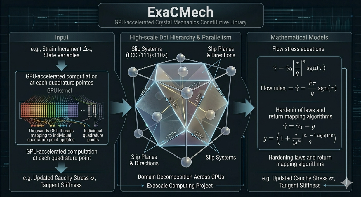
The Problem ExaCMech Solves#
Crystal plasticity finite element codes spend a large fraction of their time doing one thing: the constitutive update. Given a material’s current state (its crystal orientation, internal hardening variables, elastic strain) and a prescribed deformation over a time step, compute the resulting stress and update the material state. This has to be done at every quadrature point in the mesh, which in a production micromechanics simulation means evaluating physically complex, iterative nonlinear equations simultaneously at tens of millions of points. For the problem to be tractable at scale, those evaluations need to run on the GPU, and the models need to be structured in a way that maps naturally to how GPUs actually execute work.
ExaCMech was built to make that possible. It is an open-source library of constitutive models for crystalline materials, covering the slip-system geometry, dislocation kinetics, and thermoelastic response needed to simulate metals like copper, steel, and titanium at the grain scale. The library is designed primarily to be embedded in host finite element codes, most notably ExaConstit, but its interface is clean enough that it can also be driven standalone for material point studies, parameter fitting, or model development. The design has evolved considerably over the years, and the story of how it got there follows closely the scientific demands that pushed it.
The Original Design#
The original ExaCMech covered the Voce and Kocks-Mecking Balanced Dislocation Density (KMBalD) hardening models with their associated slip kinetics, and it supported FCC, BCC, and HCP crystal structures from the start. The structure was a virtual base class defining the interface host codes interacted with, a factory function returning model instances by name, and physics living inside templated classes assembled from slip geometry, kinetics, and thermoelastic components. For that initial scope this worked well.
KMBalD in particular was designed from the beginning to be a broadly useful reference model. It tracks a single dislocation density as the hardening state variable and handles strain rates spanning the quasi-static regime through the high-rate phonon-drag-dominated regime in a single unified formulation, transitioning smoothly between regimes without requiring the user to specify which one they are in. That robustness across a wide range of conditions has made it the reference model for FCC, BCC, and HCP applications throughout the library’s development. One of the first things added alongside the library itself was a tool to actually test it.
The Miniapp: Testing Performance and Code Structure#
The standalone miniapp was added early in ExaCMech’s life as both a usage guide and a performance benchmarking tool. The original miniapp ran a fixed loading case for a hardcoded material, which was enough to verify the library was working and to get a baseline GPU versus CPU timing. That turned out to be useful almost immediately: as the library’s internal structure changed, the miniapp gave a concrete way to see whether a code change had actually improved GPU throughput or just looked cleaner. It became a standard part of the development loop: make a change, run the miniapp, check if it got faster.
Over time the miniapp was expanded to use the model introspection system and accept runtime configuration, making material choice, loading condition, time step, and execution backend all controllable through a simple input file with no recompilation required. This is what made it genuinely useful for comparing across backends: running the same loading case on CPU, OpenMP, and GPU with a single input file change is how you measure real speedup numbers in a controlled way. One diagnostic it tracks that proves consistently useful is the distribution of nonlinear solver iteration counts across all material points, reported at each time step. A tightly clustered, low-count distribution indicates a well-conditioned model under a manageable load. A long tail of high-iteration-count points, or a non-zero count of failed points, is an early warning that something about the parameter set, time step size, or loading condition is pushing the solver into difficult territory, and catching that in a miniapp run is much better than discovering it hours into a production finite element simulation. It was also through the miniapp that I worked out one of the library’s more counterintuitive performance decisions.
Performance Portability and the Fused Kernel#
The hardware portability strategy in ExaCMech is organized in two complementary layers. At the outermost level, the library presents a simple, stable interface to host codes: supply material parameters, hand off data, tell it where to run. The host code never needs to know what crystal structure, kinetics law, or hardware backend sits underneath. Beneath that interface, RAJA and CHAI handle the actual dispatch. RAJA lets the per-material-point compute loop be written once and dispatched to serial CPU, OpenMP, CUDA, or HIP purely through compile-time configuration, with no platform-specific branches in the physics logic. CHAI manages the memory side, ensuring model data is accessible from within GPU device kernels without manual management of data movement. For CPU-only builds, the GPU machinery degrades gracefully.
One deliberate design decision deserves explanation because it goes against conventional GPU programming advice. The standard guidance is to decompose work into many small, focused kernels. ExaCMech keeps the entire per-material-point constitutive update (including the iterative nonlinear solve) as a single fused unit of work per GPU thread. As I worked out during the SNLS batch solver experiments using the miniapp, the fused approach is about 2.5x faster than breaking the same work into multiple kernel launches. Kernel launch latency adds up quickly, fusing lets the compiler optimize the full computation as one unit, and the intermediate values generated during the iterative solve are local to one material point: writing those to global GPU memory between launches and reading them back would introduce bandwidth costs no amount of kernel-level simplicity could offset. With the performance story settled and the initial model set working well, the scientific ambition that drove the next phase was pushing the model physics considerably further.
Building Out the Advanced Models#
The Orowan-type dislocation density model family was the first major push beyond what the original library supported. Where KMBalD tracks a single aggregate dislocation density, the Orowan models evolve individual dislocation densities on each slip system, both mobile and total populations, allowing hardening interaction between slip systems to be modeled with a full interaction matrix rather than a single isotropic parameter. This is a meaningful step in physical fidelity, enabling predictions of texture and hardening evolution that simpler single-variable models cannot capture.
Developing the Orowan models took roughly a year and a half of sustained iteration. The challenge was not primarily the derivative terms. Working those out on paper for each model form took at most a few days each time, and while getting every partial derivative right required care, that was not where the time went. What really consumed the effort was making the model numerically robust across the full range of loading conditions and parameterizations I was throwing at it. The governing equations needed to be the right ones, the slip kinetics needed to be stable under conditions that pushed earlier formulations into failure, and finding parameterizations that worked well across different use cases required a lot of trial and refinement. The model ultimately converged on a form that borrows slip kinetics from the KMBalD framework and integrates model forms from the literature in ways that provided the robustness I was after. This same process of debugging difficult convergence behavior under extreme conditions is also what led SNLS to develop its hybrid solver: the standard trust-region dogleg was sometimes not enough, and the search for an alternative is what produced the Powell-inspired hybrid implementation.
The MD-informed BCC formulation is the most structurally novel model in the library. Rather than treating slip planes as fixed crystallographic entities, it recognizes that in BCC metals at low temperatures and moderate to high stresses, the plane on which a dislocation actually glides is not fixed. Dislocations move in a continuous zone of possible planes sharing the primary slip direction, and which plane is active at any instant depends on the current stress state. The model computes the active slip plane dynamically at each constitutive call and tracks the orientation within that zone as a material state variable, a meaningful departure from how BCC plasticity has traditionally been modeled, motivated directly by insights from atomistic simulations that fixed-plane models cannot reproduce. Getting this one stable across a wide range of conditions required the same kind of iterative model form exploration the Orowan work did. By the time both were in reasonable shape, it had become clear that the process of iterating on model physics needed better tooling.
Python Bindings: Debugging the Hard Problems#
The Python bindings for ExaCMech grew directly out of the Orowan model work. When nonlinear solver failures are happening inside a complex GPU kernel, understanding why is difficult. Adding debug instrumentation to the C++ code, rebuilding, and running again to probe different aspects of the convergence behavior is slow and cumbersome. What I needed was a way to drive the constitutive model interactively, examine intermediate state, and experiment with different solver strategies without touching the C++ build.
The first layer of Python bindings exposes the standard constitutive interface: construct a model by name with a parameter array, query state variable names and initial values, and run material point simulations through a simple solve call. This covers stress-strain curve generation, parameter sensitivity studies, and comparison against experimental data. The second layer, more developer-focused, exposes the internals of the constitutive update more directly, allowing access to components of the batch update otherwise hidden behind the primary interface. It was designed specifically for exactly the kind of solver debugging the Orowan work required: examining intermediate state, substituting different solution strategies, and probing convergence behavior on realistic material data without rebuilding. This tooling made iterating on difficult model forms considerably more tractable. The Python work also happened to coincide with a broader refactoring effort in ExaCMech, and the knowledge from that refactor is what then opened the door to the JAX implementation.
The Refactoring Work#
A year or two after the Python bindings were in place, I found myself at a point where the library had accumulated enough complexity that continuing to push it forward productively required stepping back and cleaning house. The place I started was the physics code itself, because that was where the day-to-day friction was most felt. The original single-point constitutive update was a dense monolith where EOS evaluation, hardness state update, nonlinear problem setup, solver invocation, solution extraction, tangent stiffness computation, and stress rotation were all interleaved. The code was correct, but understanding what any particular section was doing required holding the entire surrounding context in mind. A common complaint from new contributors was that they could not productively work on it without a guided tour from an original author, which is not a sustainable way to grow a library. The refactored version pulls the logical stages apart into clearly named, independently understandable pieces: preprocessing separated from the solve, the problem state as a proper documented object, multiple problem formulations sharing well-defined common infrastructure, the tangent stiffness documented with the mathematical derivation it implements. None of this affects runtime performance, but it substantially reduces the time a new developer spends before being able to contribute.
Going through the physics code that carefully also made it easier to see where other structural problems had crept in. Build times had become painful. The original factory and all its model instantiations lived in a single monolithic header file, and because GPU compilers generate and optimize a complete copy of every computational method for each template configuration, builds were taking an unreasonable amount of time and holding up projects depending on the library. The fix was to keep a lean header as the public factory interface while moving the actual instantiations into source files organized by crystal symmetry, one for FCC, one for BCC, and one for HCP. BCC required further splitting given the number of model variations it had accumulated, with the Orowan variants getting their own translation units separated by slip system count. Each of those files is its own translation unit so the build system parallelizes their compilation naturally. Adding a new model means adding it to the appropriate existing source file for its crystal symmetry type, with further reorganization only warranted if a particular group grows large enough to become a build bottleneck again. Similarly, once the internal structure was cleaner, it was easier to see that the code offered essentially no support for a question every host code needs to answer when selecting a model: how should I set up my data arrays, and where do the various quantities live? The solution was a model introspection system that returns a complete named map of everything a downstream user needs, covering parameter counts by sub-component, total state variable count, and integer starting positions of every named quantity, all extracted directly from the model’s compile-time structure so it is always consistent with what the model actually uses.
Working through all of this gave me a much clearer mental model of how the library was structured end to end, and it was that clearer picture of the internals that made the JAX implementation tractable shortly after.
JAX ECMech: Prototyping Without the Derivative Tax#
After working through the Orowan and MD-informed BCC models, the pattern of what made new model development slow was clear. Implementing the rate equations for a new kinetics law is not the hard part. What slows things down is the combination of getting the analytical derivatives right and verifying that the model behaves physically sensibly under all the conditions you care about. Even when the derivatives only take a few days to derive, getting them all the way correct and then discovering the model form still doesn’t behave the way you want in some regime means starting over, and repeating that loop in C++ is slower than it needs to be.
The JAX port of ExaCMech’s core crystal plasticity model was built to make that early iteration phase faster. Because JAX can automatically differentiate through Python implementations, a developer can implement only the rate equations and immediately obtain derivatives that are by construction exactly consistent with those equations. Running material point simulations to verify that a new model form produces physically sensible stress-strain behavior takes a few dozen lines of Python. The JAX implementation includes a Python port of the same trust-region Newton solver used in the C++ library, so convergence behavior between the two is directly comparable. Once a model has been prototyped and validated, the analytical derivatives for the production C++ implementation can be checked against JAX’s output as a principled correctness verification. This validation path has caught subtle derivative errors that finite-difference checks at a single point would have required unreasonably tight tolerances to detect. More than the correctness checking, though, it is the speed of early exploration that matters: decoupling the question of whether a physical idea is worth pursuing from the full cost of implementing it in production C++ makes it realistic to try more things.
Material Model Coverage and State#
The library’s model coverage spans FCC, BCC, and HCP crystal structures with several kinetics choices at different levels of physical fidelity. For FCC metals, ExaCMech provides a Voce hardening model with power-law kinetics, a nonlinear Voce variant, KMBalD for physically based rate-dependent response, and the Orowan-type model with per-slip-system hardening evolution. BCC metals receive the most extensive treatment: the standard Schmid-law formulation with 12, 24, or 48 active slip systems; a non-Schmid formulation capturing the twinning versus anti-twinning asymmetry important for materials like molybdenum and tungsten at low temperatures; and the MD-informed dynamic slip plane model. HCP metals are supported through KMBalD with a 24-system slip geometry covering basal, prismatic, and pyramidal slip families.
Across all models, each material point carries a full state history: crystal orientation as a unit quaternion, deviatoric elastic strain, per-slip-system shear rates, hardening variables, and diagnostics including effective shear strain rate, accumulated plastic strain, flow strength, and the nonlinear solver iteration count. Surfacing that last quantity as an accessible state variable rather than a buried solver internal is a deliberate choice, because it is precisely what tells a simulation engineer which material points are numerically difficult and whether a time step or parameter adjustment is warranted before committing to a production run.
Looking at the Bigger Picture#
When I look at ExaCMech now compared to where it started, the growth reflects a consistent pattern: each tool that was added existed because a real problem made it necessary. The miniapp was there from early on to measure whether code changes actually helped. The Orowan and MD-informed BCC models came from scientific questions that simpler models could not answer, and the iterative work to get those models numerically robust across a wide range of conditions is what produced the Python bindings, the SNLS hybrid solver, and eventually the JAX implementation. The refactoring work and JAX came together at the end of that arc, with the cleaner mental model of the library’s internals that the refactoring produced being what made the JAX port tractable. None of those were designed in advance. They accumulated in response to what the work actually demanded.
That chain of cause and effect is also what I find most satisfying about the library’s trajectory. The modernization work I did on SNLS opened the doors for this refactoring effort, and the lessons from both then fed directly into ExaConstit’s major refactoring that followed. The infrastructure that makes ExaCMech extensible today was earned through the process of pushing the models further. The JAX port and Python bindings mean that exploring a new model form no longer requires going all the way through the C++ implementation to find out whether the underlying physics idea is worth pursuing. The architecture built up through the refactoring work means adding a new model is a matter of implementing a well-defined interface rather than understanding the entire codebase. Crystal plasticity constitutive modeling at GPU scale should not require years of systems programming experience to experiment with, and ExaCMech is considerably closer to that than it was when I first started working on it.