Where ExaConstit Came From#
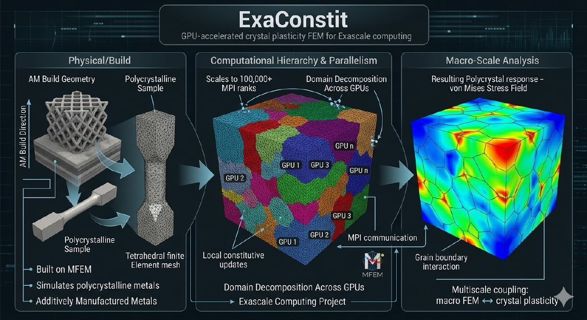
When I joined the ExaAM project at LLNL, the project needed a crystal plasticity finite element code that could run on GPUs at scale. ExaAM is a DOE Exascale Computing Project effort to model metal additive manufacturing from the melt pool all the way up to the part scale, and the part that connects microstructure to part-scale mechanical response requires simulating thousands of individual grains with their own crystal orientations, phases, and slip systems. At the time, no open-source code existed that could do this on GPUs in a serious way. Most comparable codes either had no GPU support or treated it as an experimental add-on that barely worked. So we built ExaConstit from scratch with GPU execution as a first-class target from day one.
The central question ExaConstit answers is: given a real microstructure with all of that grain-level complexity, what are the bulk mechanical properties, how do stresses and strains distribute across grains, and how does plasticity evolve over a loading history? This kind of simulation underpins materials qualification, connects microstructure generation tools to part-scale structural codes, and enables direct quantitative comparison against synchrotron diffraction experiments. When ExaConstit was first publicly released, it was among the first open-source solid mechanics codes to demonstrate running crystal plasticity simulations on GPUs at meaningful scale, and GPU-accelerated runs have since achieved speedups of 15-25x over CPU for crystal plasticity workloads. Getting to that point required not just implementing the physics, but working through years of interaction with leadership computing facilities that shaped a lot of what the code looks like today.
Getting Off the Ground: Install Scripts and Configuration#
The install scripts that ship with ExaConstit did not exist at the beginning. They grew out of a practical need that emerged over years of working with the Livermore Computing and Oak Ridge Leadership Computing staff during the ECP. As part of the exascale push, I was regularly filing bug reports with AMD and NVIDIA for issues encountered in GPU builds. To get those bugs taken seriously and fixed, I needed to be able to hand the computing facility staff a way to install the code and reproduce the problem in a minimal example, quickly and reliably. That required making the full dependency chain (MFEM, RAJA, Umpire, CHAI, ExaCMech, Hypre, METIS) buildable in a predictable way with a single script.
That process turned out to matter beyond just bug reproduction. One of the issues I was filing related to the performance of small matrix operations on AMD GPUs. I had benchmarked these against MAGMA’s fast batch GEMV implementation for small matrices (where N and M are both at most 32), showed the performance gap explicitly, and this comparison is what eventually led AMD to implement their own fast batch GEMV for that size range. Getting a GPU vendor to prioritize a specific kernel optimization requires being able to clearly demonstrate what performance is achievable and what the current gap is, which meant having a reproducible, well-documented setup. The install scripts were the byproduct of learning to do that well.
Configuration for actual simulations is handled via TOML files that control everything from mesh paths and boundary conditions to material model selection, assembly strategy, and visualization output. No recompilation is required to change any of these, and a legacy-to-modern conversion script handles migrating older input files forward as the config schema evolves. The combination of install scripts and TOML-based configuration reflects a conviction that the barrier to getting a first simulation running should be as low as possible, because a code that works brilliantly but takes a week to set up will not get used. With onboarding handled, the underlying portability question shapes everything else.
Performance Portability: One Codebase, Many Backends#
The GPU portability strategy is built around two complementary libraries: MFEM for finite element data structures and operator abstractions, and RAJA for portable loop execution. Compute kernels are written once using a backend-agnostic abstraction and compile to sequential CPU, OpenMP-threaded, CUDA, or HIP targets depending on the selected backend. The same physics and assembly code runs on a developer’s laptop, an NVIDIA V100 cluster, and an AMD MI300A system without a single platform-specific branch inside the physics logic. Memory management across the host-device boundary is handled through MFEM’s device-aware data types, which track whether data is currently valid on host or device and manage transfers lazily to avoid unnecessary round-trips. The result scales across thousands of MPI ranks on leadership-class machines while maintaining competitive single-node CPU performance through the same code path. That portability is what makes ExaConstit practical to maintain and deploy across a landscape of rapidly evolving hardware, but it sits on top of a finite element framework that needed careful structure to support it.
The FEM Framework: Separation of Concerns at Scale#
At its core, ExaConstit solves a nonlinear quasi-static mechanics problem at each time step using Newton-Raphson iteration. Each Newton step requires computing a global residual vector and a tangent stiffness operator assembled from local contributions at every quadrature point across the mesh. The framework is structured so that three concerns are cleanly separated: time-stepping and nonlinear solve logic, finite element assembly machinery, and the constitutive model. The assembly layer communicates with material models through a narrow, well-defined interface: it hands off local deformation state at each quadrature point and receives back updated stress and a material tangent, with no knowledge of what is happening inside the constitutive model. This separation means solver strategies, assembly methods, and material models can all evolve independently, which has proven essential as the code has grown.
MFEM provides three assembly strategies selectable at runtime: full assembly (traditional global sparse matrix), element assembly (only element-level matrices, no global formation), and partial assembly (fully matrix-free operator actions). Element assembly is the GPU sweet spot for quadratic or lower-order elements, hitting a favorable balance between memory bandwidth and compute. Partial assembly becomes advantageous at high polynomial orders where the operator-versus-storage tradeoff flips. For near-incompressible plasticity common in metal forming, a B-bar formulation modifies the volumetric strain interpolation to prevent pressure locking without disrupting the assembly structure. As the code grew to support multiple materials and an expanding contributor base, the clean architectural separation that worked at small scale needed to be reinforced at the data management level too.
Refactoring for Clarity: SimulationState#
As ExaConstit matured from a research prototype into a production code with multi-material support, more complex post-processing, and a growing developer community, the original data management approach became a bottleneck, not in performance but in comprehensibility. Data was passed around through a mix of raw pointers and references, ownership was implicit, lifetimes were difficult to reason about, and adding a new feature often meant threading a new pointer through multiple layers of function arguments just to reach the place where the data was actually needed. Contributors understandably found this frustrating to navigate.
The refactoring effort introduced SimulationState as the single authoritative owner of all simulation-wide data: mesh, finite element spaces, material state at quadrature points, boundary condition configurations, orientations, and the material model registry. Rather than passing raw pointers to individual pieces of data through the call stack, components accept a std::shared_ptr<SimulationState> at construction time and hold onto it for their lifetime. This shift to shared ownership made lifetime reasoning trivially simple: no component can outlive the data it depends on, no raw pointer is left dangling when an object is destroyed, and the code expresses ownership intent clearly without manual bookkeeping.
This was not a cosmetic change. Multi-material support, where different mesh regions carry different constitutive models, different state variable counts, and different quadrature data layouts, would have been extremely difficult to implement correctly against the original data management approach. With SimulationState centralizing everything and providing a per-region query interface, adding a new region is a configuration-level change rather than surgery on data routing throughout the code. Centralizing the data also exposed a subtler problem: the standard quadrature data abstractions in MFEM weren’t quite the right shape for multi-material use.
Partial Quadrature Spaces and Functions#
Standard quadrature spaces and functions in MFEM are defined over the entire mesh. In a multi-material simulation, this is both wasteful and conceptually wrong: a crystal plasticity model for Region A has nothing to say about the quadrature points in Region B, and allocating and managing data for the full mesh when only a subdomain is relevant forces unnecessary bookkeeping and inflates memory use.
The solution was a new pair of data abstractions: PartialQuadratureSpace and PartialQuadratureFunction. These define quadrature spaces and their associated data over arbitrary subsets of mesh elements, such as material regions or any element grouping that makes physical sense. A PartialQuadratureSpace holds a local-to-global element mapping so subdomain-local indexing always translates correctly to global mesh indices, and PartialQuadratureFunction builds on this to store and operate on field data only for the relevant elements. Constitutive model data for each material region is natively scoped to that region, and post-processing operations only touch that region’s data. This design proved general enough that it is in the process of being upstreamed to MFEM proper, which means the broader MFEM community will be able to use subdomain-native quadrature data structures in any finite element code built on the library. With the data structures in better shape, the next question was how to make the material model interface as flexible as possible.
Material Model Flexibility: From ExaCMech to Dynamic UMATs#
A simulation code’s longevity depends heavily on how easy it is to plug in new material models without touching the FEM infrastructure. ExaConstit approaches this through two parallel strategies. The first is deep integration with ExaCMech, which provides physically-based models covering FCC, BCC, and HCP crystal structures with various hardening laws and slip kinetics that run natively on the GPU. The constitutive update executes in parallel across all quadrature points without requiring data to leave the device.
The second strategy is the UMAT interface: the standard constitutive model calling convention from Abaqus. Any model conforming to that interface, written in Fortran, C, or C++, can be integrated. Critically, UMATs can be loaded at runtime as shared libraries via dlopen rather than compiled into the executable, so researchers can develop, iterate on, and deploy new material models without touching ExaConstit’s build system at all. The loading strategy is configurable: persistent loading, lazy loading, or reload-on-setup for debugging. Multi-material simulations where different mesh regions use entirely different model types are handled through a composite design pattern that presents a single unified model interface to the rest of the framework, so the FEM assembly machinery does not know or care whether it is talking to ExaCMech, a UMAT, or some combination of the two. Once the physics are running correctly, the next challenge is making sure you can actually see what is happening.
Logging, Diagnostics, and Profiling#
In an MPI simulation, stdout from dozens or thousands of ranks is often interleaved or suppressed in ways that make debugging material model setup or convergence issues painful. ExaConstit’s unified logger operates in two modes: a persistent tee mode that duplicates all stdout and stderr to a timestamped log file throughout the simulation, and a capture mode that temporarily redirects output from a specific code region to its own named file. This capture mode is used extensively during material model initialization, so each model’s setup output goes to a per-region, per-rank log file rather than flooding the main simulation log. The logger uses RAII semantics to guarantee stream buffers are always restored even if exceptions occur, handles GPU printf buffer flushing before ending a capture session, and coordinates across MPI ranks so that only designated roots produce summary output. Caliper integration provides hardware performance counter and timing data when profiling builds are needed, and compiles away completely in production builds with zero overhead. With diagnostics covered, the last major piece is getting useful results out.
Post-Processing: Multi-Material Output#
Post-processing for multi-material simulations requires some care about what is being computed and where. In ExaConstit, the flow goes from the global mesh and its associated PartialQuadratureFunctions down to per-region ParSubMesh representations, not the reverse. Each material region is represented as a proper parallel sub-mesh containing only its elements, with its own set of grid functions and data collections. This per-region decomposition is what makes visualization of individual material responses clean in tools like VisIt or ParaView, and it is a natural consequence of the partial quadrature space design.
The volume-averaging system computes volume-weighted averages of the full Cauchy stress tensor, deformation gradient, elastic strain, equivalent plastic strain, and plastic work at each output step, at both per-region and global levels. Simulation time and element volumes are captured directly in these output files rather than as separate metadata, so the data is self-contained for downstream analysis. New volume-averaged quantities can be registered with the post-processing driver through a simple function registration interface, and they automatically inherit the caching, output formatting, and MPI coordination logic already in place. One particular output capability deserves its own section because it connects directly back to the experimental work that motivated a lot of this project in the first place.
Lattice Strain Analysis: Connecting Simulation to Experiment#
One capability I wanted in ExaConstit from early on, motivated directly by my PhD work, is the ability to simulate what a powder diffraction experiment would measure on a given microstructure. During a synchrotron diffraction experiment, only grains oriented so their crystal planes satisfy the Bragg condition for a given scattering vector contribute to a measured peak. ExaConstit identifies which simulated grains fall within that crystallographic fiber, computes the volume-weighted average elastic strain projected along the scattering direction, and produces synthetic lattice strain versus load curves directly comparable to experiment.
The implementation exists in two forms with different capabilities. The non-situ implementations currently support FCC, which was the original use case and where most of the validation work has been done. The in-situ version is the more general implementation, supporting all eight Laue groups (cubic, hexagonal, trigonal, rhombohedral, tetragonal, orthorhombic, monoclinic, and triclinic) through a unified symmetry operation framework. For very large simulations where storing full per-element field data at every time step is not feasible, the in-situ path writes only the aggregated per-HKL lattice strain values directly during the simulation, eliminating the I/O bottleneck entirely. Analysis is performed at the per-region level in both cases, so in a multi-phase simulation each material’s diffraction response is tracked independently. The hot-path computations were rewritten as a Rust crate with Python bindings via PyO3, the xtal_light_up library, giving native execution speed with an unchanged Python interface. The ability to compare simulation directly against synchrotron measurements was central to the scientific goals of this project, and the workflow integrations connect those goals to real production pipelines.
Workflows: Parameter Optimization and ExaAM#
ExaConstit ships with two major workflow integrations. The first is a multi-objective material parameter optimization workflow built around NSGA-III, a genetic algorithm suited to simultaneously matching multiple experimental datasets such as stress-strain curves at multiple strain rates or temperatures. The workflow integrates with LLNL’s Flux job scheduler, launching ensembles of ExaConstit runs as parallel jobs and aggregating results back to the optimizer automatically.
The second is the ExaAM workflow, the one ExaConstit was originally built for. ExaCA, a cellular automata code for simulating solidification microstructures during laser powder bed fusion, generates grain structures that feed directly into ExaConstit as input meshes. ExaConstit then computes the mechanical response of those as-built microstructures, providing homogenized constitutive data for part-scale structural models and anisotropic yield surface development. This workflow spans the full process-structure-property chain, enabling questions like “how does variation in laser scan speed propagate to uncertainty in yield strength?” to be answered quantitatively rather than assumed. Making these workflows available as part of the code, rather than as internal-only scripts, connects to something I feel fairly strongly about.
On Open Source and Scientific Culture#
There is a personal dimension to how ExaConstit is developed and shared that is worth being direct about. My own PhD research was built on a code that was closed source at the time. My adviser retired partway through, and only after I had finished as his last student did the code eventually become available. That experience shaped a strong conviction: the broader research community should not have to recreate infrastructure that already exists simply because it was never made accessible. Researchers should be able to see how things are implemented, how material models are parameterized, and how large uncertainty quantification studies are actually structured, rather than just read descriptions of them in papers.
That conviction shows up throughout ExaConstit: in the install scripts that grew from bug filing into a genuine onboarding tool, in the TOML-based configuration that makes simulation setup readable without reading source code, in the optimization and UQ workflows shipped alongside the solver rather than kept as internal tools, and in the postprocessing scripts that close the loop from raw simulation output to the curves and figures researchers actually need. The major refactoring that gave ExaConstit its current architecture (SimulationState, the partial quadrature space abstractions, and the restructured post-processing system) was made possible by the lessons learned from the modernization work on SNLS and ExaCMech that came before it. Each of those efforts taught something about how to do this kind of refactoring at scale, and ExaConstit benefited from all of it. Making a code performant is one kind of contribution to the community; making it genuinely usable and understandable is another, and I would argue the latter is in some ways harder and less rewarded. ExaConstit tries to take both seriously.